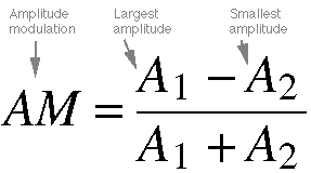
Equation 11.1. This equation calculates the factor of amplitude modulation (AM). The factor is determined by taking the difference between the maximum (A₁) and minimum (A₂) amplitudes, and dividing by the sum of these two amplitudes. There are two extreme cases: (1) when A₂ = A₁, there is no (0) modulation of the carrier frequency, and (2) when A₂ = 0, there is 100% modulation. In the latter case, the carrier frequency has a amplitude of zero, which is a violation of amplitude modulation. In most cases, the amplitude modulation factor is below 50 percent.

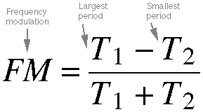
Equation 11.2. The method for determining the frequency modulation (FM) factor is quite similar to that of determining amplitude modulation. In this case, T₁ and T₂ are the maxmimum and minimum periods, respectively. In the case where T₂ = 0, the frequency (1/T) momentarily approaches infinity, which is a violation of frequency modulation.

Equation 11.3. To determine the mean value of cyclic variable of vocal fold vibration, one should calculate it in the standard mean calculation method -- i.e., sum all (N) instances and divide by the number of instances (again, N).

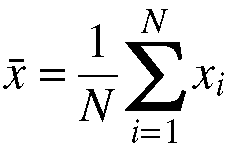
Equation 11.4. Mathematically, the above equation is equivalent to equation 11.3. Sigma (S) is the Greek letter equivalent to the Roman letter S. In mathematics, the sigma notation represents summation. Below the sigma is the expression i=1, which the initial value of i. N, which appears above the sigmal, is the final value of i. Following the sigma is the expression to be summed for all values of i. Hence, the sigma and the expression following it in this case represent the sum of all values from x₁ through x_N. This sum is then divided by the total number of instances (N) to determine the mean or average value. When written out in its entirety, the equation is exactly what is seen in equation 11.3.

Equation 11.5. To determine the zeroth-order perturbation of the ith cycle, we need to take the difference between the value of the ith cycle and the mean value. The resulting value is represented by p_i

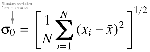
Equation 11.6. Standard deviation is an important concept in the realm of statistics. Its value is an indicator of the deviations that the various instances (in this case, cycles) display from the mean as a group. Standard deviation is calculated by summing the squared value of the perturbation, dividing by the number of instances, and then taking the square root of that value. Standard deviation is normally represented by a lower case sigma (s). A subscript of 0 represents that this standard deviation is of the zeroth order.

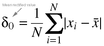
Equation 11.7. Another commonly calculated statistical value is the mean recified value. This is determined by taking the sum of the absolute value of the pertubations, and then dividing by the total number of instances. Note the difference between this equation and the equation to determine the mean (equation 11.3). The vertical bars indicate absolute value, which is always the non-negative representation of a value. (e.g., the absolute value of -3 is 3.) Mean rectified value is normally represented by a lower case lambda (l). As in equation 11.6, a subscript of 0 represents zeroth order.

Equation 11.8. First-order perturbation is a ramp -- in other words, it is the local linear trend made to the current point from the last. The value k represents the overall mean rise per cycle, and the expression (x_i - x_i-1) is the rise between adjacent cycles.

Equation 11.9. We can apply the standard deviation technique explained in Equation 11.6, although we must be careful. As we are now analyzing the intervals between cycles rather than cycles themselves, we have one less value to work with. (A simple analogy can be made -- while you have five fingers, there are only four spaces between any two adjacent fingers.) The initial value of i is hence set to 2, as we must account for the term x_i-1 equalling x₁ in this case, and the final value of x_i will be x_N. Hence, when taking the standard deviation, while we square the perturbation, we divide by one less than the number of cycles, and then again finally take the square root. This time, a subscript of 1 is used to indicate the first-order standard deviation.

Equation 11.10. The first-order mean rectified value is calculated in a similar manner as equation 11.7, taking the same considerations in mind as done with first-order standard deviation. Essentially, this value is equal to the sum of the absolute values of the ramps divided by the number of intervals. A subscript of 1 indicates first-order.

Equation 11.11. The last example of perturbation is the second-order case, which represents removing a local linear trend (rather than calculating it). This is calculated using the equation above (adopted from Pinto & Titze, 1990).

Equation 11.12. To determine second-order mean rectified value, we first need to divide the perturbation function by two -- this is done such that the scale is similar to the first-order measures. As each pertubation now spans two intervals (requiring three points), the range for i is reduced again by one. This time, the range is from 2 (where the minimum value of x_i-1 is equal to x₁) to N-1 (where the maximum value of x_i+1 is equal to x_N). We also reduce the divisor by 1 to N-2 to reflect this change. From there, the standard approach of summing absolute values and dividing by the number of instances should be clear. Again, the subscript 2 represents second-order.

Equation 11.13. Finally, standard deviation techniques are applied to half of the expression in 11.11, again for scaling reasons. The range and divisor are used for the same reason as for the mean rectified value.